

A driver-based model that answers what happens to CAC and margin if you raise spend 20 percent, before you spend a dollar.
A driver-based forecast you own, built from your own numbers. Change one input, Meta spend, AOV, repeat rate, and blended CAC and contribution margin recalculate in front of you. No BI seat, no analyst queue. About 30 minutes to build once, then it is yours to pressure-test forever.
Below is a full worked example: the exact model, run end to end on a ~$20M/yr DTC brand. Then the steps to build your own.
Here's the spreadsheet 👇
https://docs.google.com/spreadsheets/d/1-9yLvy1zMLoc_NKbsy22R2exgfKod7nn4ctuqf_6b1k/edit?usp=sharing
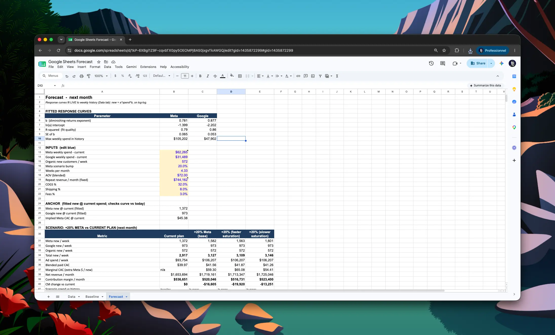
Here is what the finished model produced, so you know what you are building toward.
Baseline (per month, from the last 13 weeks of actuals):
Response curves fit to the brand's own weekly history (new = a × spend^b, fit on log-log):
The b below 1 is diminishing returns, measured, not assumed. And the model reproduces the CAC the brand actually runs today ($45 on Meta), so the curve is anchored to reality.
The scenario, raise Meta 20% next month, shown as a band, not a single number:
                          current    +20% Meta (base)   band (low / high)
Total new / week          2,917      3,127              3,109 / 3,146
Blended paid CAC          $39.97     $41.56             $41.87 / $41.26
Marginal CAC (next $/new) n/a        $59                $65 / $54
Contribution margin / mo  $536,651   $520,046           -$19,920 / -$13,251
CM change vs current      0          -$16,605           contribution-NEGATIVE
The read: pushing Meta 20% harder costs this brand roughly $13k to $20k of contribution margin next month, and the very next dollar on Meta costs about $59 to acquire a customer worth less than that. The spreadsheet says do not do it, on the brand's own numbers. That is the whole point.
A spreadsheet with three tabs:
Claude builds all three as an Excel file, you open it in Google Drive, and it becomes a live Google Sheet. Change any input and the whole thing recalculates.
In Claude, open Connectors and connect the sources that feed the baseline. Shopify and Klaviyo are first-party connectors, enable and authenticate in a couple of clicks. Meta Ads and Google Ads connect through their own MCP servers, added as custom connectors. If you would rather skip that setup, a bundled connector (for example Windsor.ai or Adspirer) brings the ad platforms in through one integration.
For a channel with no connector, TikTok Shop, Amazon, a 3PL, bridge it with the Zapier MCP, pipe it into a warehouse and connect that, or drop a CSV in each time. A forecast is only as good as its baseline, so getting these sources right matters more here than anywhere else.
Give Claude this prompt:
You have access to my Shopify, Meta Ads, Google Ads, and Klaviyo. Build me an Excel file (.xlsx) called "Forecast Model" with two tabs.

Baseline tab, from the last 3 to 6 months of actuals, as a monthly run-rate:
- Net revenue by channel and blended
- Ad spend by channel
- Blended and per-channel CAC
- Contribution margin (revenue minus COGS, shipping, fees, and attributed ad spend). Put COGS percent, shipping, and fee assumptions in labeled input cells so I can edit them.
- New vs repeat revenue, and AOV

Data tab, the raw material the forecast will fit against: the last 12 months (or as much as I have) at weekly granularity, spend by channel and new customers by channel, one row per week.

Label the date range. Use live spreadsheet formulas throughout, not pasted values, so the sheet recalculates when I change an input. Note which numbers are a point-in-time snapshot from my sources.

Claude pulls the numbers and writes a real spreadsheet: labeled inputs, live formulas, and the weekly rows Step 3 needs. Download it, open it in Google Drive, and it converts to a Google Sheet with the formulas intact.
Two things to know before you build on it:
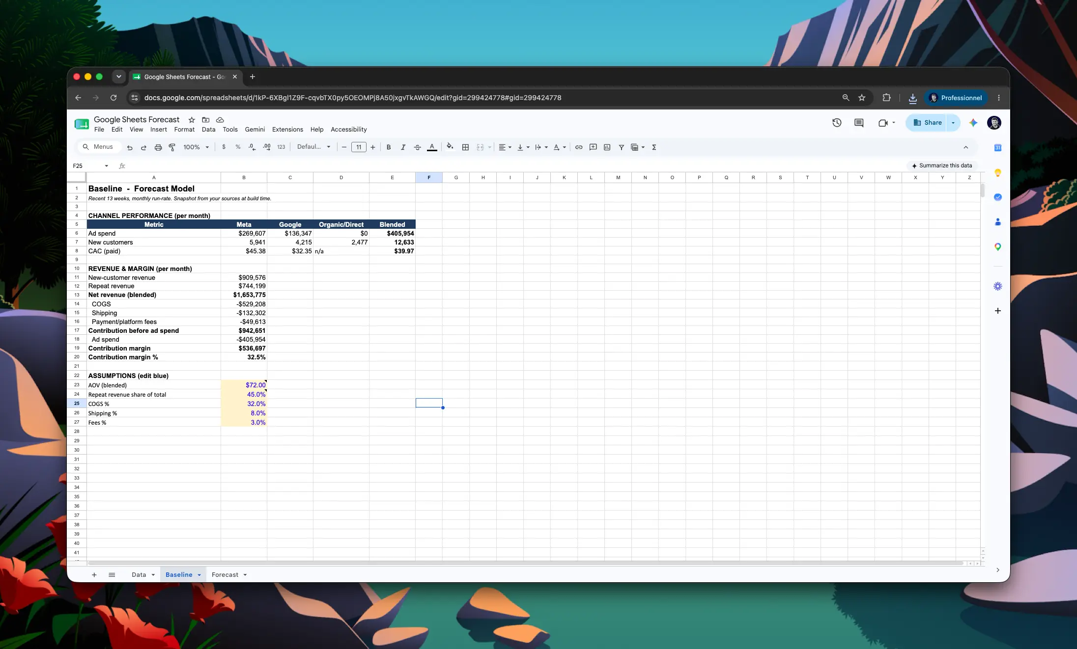
Here is the move most spreadsheet forecasts get wrong. They assume "20 percent more spend equals 20 percent more revenue," which overstates the upside every time, because ad spend has diminishing returns. The fix is not to guess the curve, it is to fit it to your own data. Monthly, your spend looks flat, but week to week it moves, and so do your new customers. That variation is exactly what a response curve is fit against. Give Claude this prompt:
Using the weekly Data tab, build a Forecast tab.

For each channel, fit a diminishing-returns response curve of new customers to spend, a concave form, new = a times spend^b, with b between 0 and 1. Fit it in-sheet with LINEST or SLOPE/INTERCEPT on the log-log data so it stays live if I edit the data, and put a, b, and the fit's R-squared in labeled cells per channel, with the date range the fit is based on. Check that each curve reproduces my actual recent CAC at recent spend; if it doesn't, flag it.

Put every other assumption in its own labeled input cell too: spend by channel, AOV, repeat rate, and my cost assumptions. Project next month's net revenue, blended CAC, and contribution margin off the fitted curves and those inputs, all live formulas.

Add a worked scenario, raise Meta spend 20 percent, beside the current plan. Two rules: (1) flag whether the new spend is inside my historical weekly spend range or extrapolating beyond it, and (2) show the result as a low / base / high band by varying b across its fit uncertainty, not a single number.
Now the model does three honest things a typed-in curve cannot: the diminishing-returns slope is estimated from your own weeks, it is anchored to the CAC you actually run today, and it tells you when a scenario is projecting past anything you have ever spent instead of pretending it knows.
Spot-check before you trust it. Confirm each channel's fitted b and R-squared actually populated with a number. A misaligned cell reference can read perfectly plausible for one channel and quietly error on another, so glance at every channel's fit, not just the first one, before you believe any scenario built on top of it.
Change any assumption and watch the outputs move. Try a few: raise Google instead of Meta, hold spend flat, push AOV. It is all in-sheet formula math, so it recalculates instantly.
Watch the band as much as the midpoint. When it is wide, the response assumption is carrying the answer and the result deserves less confidence. And watch the in-range flag: the moment a scenario turns to "extrapolating," you are guessing past your own history.
When it behaves, save the prompt, that is the asset. Because the baseline is a snapshot, you refresh it by re-running the prompt to regenerate the file, not by scheduling a live sync. Re-run at the start of the month or before a budget decision. (If you would rather have a sheet Claude writes into directly and refreshes on a schedule, that is the Cowork or Claude Code path, a different setup than this one.)
Optional, but for a forecast this is the part that decides whether you would actually move budget on the answer.
Run the version above and Claude reconstructs blended CAC, contribution margin, and new vs repeat from raw rows and your typed-in assumptions, because every tool defines them differently. The model can show that raising Meta 20 percent is contribution-negative next month, but it cannot prove the repeat behavior that would justify doing it anyway. A confident forecast on a shaky baseline is how you overspend with data on your side.
Polar removes that risk: its semantic layer defines true CAC, contribution margin, and new vs repeat once across the whole business, with spend attributed for you, so the model runs on numbers you would bet budget on, not reconstructions.
Enable the Polar MCP and swap Step 2 for:
With Polar you can also rerun the whole forecast under any of its 10 attribution models and watch the recommendation change with how you count, and reach for true incrementality where the spreadsheet's correlational curve runs out.
